Chapter 6

Revenue Forecasting

by Whitney B. Afonso

Introduction

1. Forecasting attempts to identify the relationship between the factors that drive revenues (tax rates, building permits issued, retail sales) and the revenues government collects (property taxes, user fees, sales taxes). . . . Revenue forecasts can apply to aggregate total revenue or to single revenue sources such as sales tax revenues or property tax revenues. There is no single method for projecting revenues. Rather, different methods tend to work better depending on the type of revenue. Similarly, there is no standard time-frame over which to attempt a forecast.¹

This chapter presents an overview of the primary ways in which local governments forecast revenues. Revenue forecasting is critical to quality financial management in both the short term and long run. The forecasted revenues are the foundation on which the budget is built and can dramatically alter the direction and scope of government services. In fact, it is reasonable to argue that “without exception, revenue forecasting is the most important task in budget preparation.”² Although revenue forecasting is critical, there are no clear universal rules or guidelines. There is no best forecast method, nor is there any forecast method without merit or weaknesses.

Revenue forecasting is not simply a best practice, but also a necessity. In fact, North Carolina local governments are required by the Local Government Budget and Fiscal Control Act (referred to in short as the Fiscal Control Act) to forecast their revenues. This requirement, though not explicit, is present in numerous places, most clearly in two components of the Fiscal Control Act. The first is through the balanced budget requirement: “a budget ordinance is balanced when the sum of estimated net revenues and appropriated fund balances is equal to appropriations.”³ Those “estimated net revenues” are the revenue forecasts. The law does not dictate the method of estimating those revenues, but it clearly dictates that revenue forecasting must be done. The second component states that “estimated revenue shall include only those revenues reasonably expected to be realized in the budget year,” indicating that the estimates or forecasts must be reasonable and reliable as well as justifiable.⁴

This chapter proceeds with a discussion of a potential administrative process for forecasting revenues.⁵ It then presents descriptions and a discussion of qualitative and quantitative methods, with a focus on judgmental forecasting, trend analysis, and causal modeling. After providing a selection of the different methods available for forecasting, the chapter discusses additional issues to consider in choosing the right method, highlighting many concerns and best practices.

Potential Administrative Process for Revenue Forecasting

There are many ways in which a local government can structure its process for revenue forecasting; some of these choices will depend on capacity, diversity of the local government’s revenue portfolio, and the stability of their local economy. However, there are four basic steps for creating and implementing a transparent, easily replicated (internally and externally) forecasting process. These steps are (1) create a revenue manual, (2) compile estimates for major non-departmental revenue sources, (3) compile estimates from revenue-generating entities within the local government, and (4) update all estimates.⁶ Each of these steps is consistent with North Carolina law.

Step 1: Create a Revenue Manual

The first step is to create a (or to maintain an up-to-date) revenue manual.⁷ A revenue manual is a complete list of all revenue sources. It often includes the following information for each revenue source: the statute authorizing the revenue source⁸ and corresponding restrictions; the current rate, previous rates, and collection rates; the forecast method; what elements in the local economy affect the revenue generated (or the tax base); and the groups that pay this tax (or fee). It also is critical to determine who collects the revenue. For example, is it collected by a public utility? By the state? Another aspect of revenue that is important to include is whether it is periodic (or seasonal), for example, a community pool that collects revenue only during the summer months or property taxes where the majority of tax remittance takes place during January and February. Ultimately, a revenue manual should contain information on all revenue sources and provide any data that will be helpful in understanding trends (including fluctuations) in revenue generation.

There is a great deal of diversity in the form that a revenue manual can take. One useful example is the revenue manual created by the City of Fort Lauderdale, Florida.⁹ It presents each revenue instrument, a description of it (including if the revenue is earmarked and the tax rate), historical collections, the current projection, and forecasts for the following five years. The manual also includes the legal authority that authorizes the municipality¹⁰ to implement that revenue, the fiscal capacity, and the forecast assumptions. It is a well-done revenue manual, but there may be even more information that a local government might want to include.¹¹ For a local government that has not yet created a revenue manual, the most productive place to begin is with major revenue sources and with building toward a comprehensive manual.¹²

As this chapter proceeds, it will become clear that many a local government performs individual forecasts only for major revenue sources, while it combines all minor revenue sources in a separate additional forecast or via departmental forecasts. Even if a local government generates a unique forecast for only three or four revenue sources, it is considered a best practice to create a revenue manual that includes all of the sources from which it collects revenues.

Step 2: Estimate Major Revenue Sources

In the second step, to be taken before beginning work on a proposed budget, a local government’s budget office should begin to create and/or compile estimates of major revenue sources that are not collected directly by departments.¹³ The Fiscal Control Act leaves quite a bit of discretion as to how local governments may present budgets and estimate revenues but states that the budget ordinance “shall make appropriations by department, function, or project and show revenues by major source.”¹⁴ The fact that the Fiscal Control Act dictates that local governments present forecasts of major revenue sources separately means that they must also be forecast separately, but local governments should do this regardless of legal mandate.¹⁵

It is important to forecast revenues separately because they likely have different tax bases and thus will react differently to changes in the economy. A good illustration of why major revenue sources need to be forecast separately are the two major revenue sources that North Carolina local governments rely on, sales and property taxes. Sales taxes are often estimated based on recent history but also are weighted by recent trends and anticipated fluctuations in the economic base. They are more reactive to these changes than property taxes; sales tax revenue grows more quickly with the economy and decreases more quickly than property taxes do. Therefore, it is unreasonable to believe that sales and property taxes will change at the same rate for forecasting purposes.¹⁶ In fact, it is likely that a forecaster will choose different forecasting methods for these two revenue sources.

Step 3: Ask for Departmental Revenue Forecasts

In the third step, a local government’s budget office reaches out to revenue-generating departments for their estimates of projected revenues.¹⁷ In North Carolina this can include such public entities as utilities, libraries, and parks. In addition, a budget office may ask the different departments to offer estimates under different scenarios. For example, it may be helpful to have water and sewer utilities provide estimates based on changing the levels of expected rainfall. This will help elected officials understand options, likely outcomes, and how sensitive these estimates are to assumptions.

This process may be considered a best practice in other states, but local governments in North Carolina are required to solicit these forecasts from revenue-generating departments. The Fiscal Control Act dictates that “before April 30 of each fiscal year (or an earlier date fixed by the budget officer), each department head shall transmit to the budget officer the budget requests and revenue estimates for his department for the budget year. . . . The revenue estimate shall be an estimate of all revenues to be realized by department operations during the budget year.”¹⁸

Steps 2 and 3 are broad steps that are really comprised of many sub-steps and will take place simultaneously. Some of the sub-steps within these steps are (1) Choose a time frame over which you are going to analyze the data. Considerations may include such factors as availability of data, quality of data, and the revenue source being forecasted. (2) Perform the actual revenue forecasts/projections and document them. Not just for the major revenue sources but also for “all other” revenue generators. (3) Evaluate your forecasts for how reliable they are. Reliability can be tested by doing a sensitivity analysis, where certain assumptions are relaxed and parameters (for example, population growth) are modified. If these changes have dramatic effects on your forecasted revenue, then those projections are too sensitive to your assumptions and model and are not considered very reliable.¹⁹

Step 4: Update Estimates

The quality of the forecasts will improve as more (and more recent) data are collected, so it is critical to update forecasts both before the budget is adopted and after. Thus, the final step is to monitor actual revenues and compare those numbers with projections and update forecasts accordingly. There are many potential sources of information and data that may be helpful to this process, including but not limited to, changes in laws and rates, changes to the tax base, changes to the underlying growth factors that drove the initial forecasts, and actual collection numbers.

This step is especially critical for such taxes as the sales tax, which generates revenue continuously, rather than for, say, the property tax, which is collected in one period. Thus, the property tax forecast may need to be updated in March but likely not again. Actual collections, especially those of a periodic nature, need to be closely monitored and checked against the forecasts. Comparing actual collections against the forecasts provides a budget officer with early warning if collections appear to be falling short of expectations.²⁰ This early warning provides time for more thoughtful midyear reductions if necessary.

In North Carolina, local governments can amend their budget ordinances any time after the ordinance is adopted.²¹ This is explicitly discussed in the Fiscal Control Act: “Except as otherwise restricted by law, the governing board may amend the budget ordinance at any time after the ordinance’s adoption in any manner, so long as the ordinance, as amended, continues to satisfy the requirements of G.S. 159-8 and 159-13.”²² While there are more restrictions surrounding amendments to the property tax forecasts, there is still room within the Fiscal Control Act for unanticipated events: “if after July 1 the local government receives revenues that are substantially more or less than the amount anticipated, the governing body may, before January 1 following adoption of the budget, amend the budget ordinance to reduce or increase the property tax levy to account for the unanticipated increase or reduction in revenues.”²³ Therefore, this can all be understood as the Fiscal Control Act encouraging local governments to carefully monitor their forecasts for accuracy and to update them throughout the fiscal year (FY).

How often forecasts should be updated depends on many factors, including capacity and previous stability. For example, larger counties, on average, start four months earlier (nine versus five) than smaller counties in terms of revenue forecasting. In part, as a result of this (and of capacity), they also modify their estimates, on average, three times during the fiscal year, whereas smaller counties do so, on average, 1.3 times.²⁴

Forecasting Methods

1. [Forecasting methods] range from relatively informal qualitative techniques to highly sophisticated quantitative techniques. In revenue forecasting, more sophisticated does not necessarily mean more accurate. In fact, an experienced finance officer can often “guess” what is likely to happen with a great deal of accuracy.²⁵

In determining what method of forecasting is best for a particular local government, there are two broad categories to choose from: qualitative and quantitative. Qualitative methods revolve around expert judgment, do not rely heavily on data, and often do not clearly lay out how the final forecasted numbers were estimated and what underlying assumptions drove them, whereas quantitative methods rely heavily on quantifiable data. Ideally, the assumptions that are used to model and categorize the relationships between variables and historical values are clearly identified. Due to their technical nature, quantitative methods are also often able to present margins of error for the forecasts, revealing the level of certainty and reliability of those estimates.

There are many ways to forecast revenues. In this chapter, the most common methods used by local governments are discussed, but the discussion is by no means exhaustive. A list of resources that provide more information on additional methods is presented at the end of this chapter.

Qualitative Methods

Qualitative forecasting relies on the expertise of an individual or a group for forecasting revenue. This may mean that a local government has an internal expert (professional) whose judgment can be trusted, for example, a budget director or a person from the agency administering the tax/fee. It is also common for local governments to solicit assistance from outside experts, such as professors, economists, business people from the community, or consultants. There are two primary types of qualitative forecasting: judgmental and consensus.

Judgmental Forecasting

Judgmental forecasting, the most common form of forecasting used by local governments, involves a single individual estimating “likely” future conditions. This can lead to very good results, especially when the forecaster has experience as well as expertise with historical trends, the state of the economy, and other factors likely to affect the tax base. “Judgmental approaches tend to work best when background conditions are changing rapidly. When economic, political or administrative conditions are in flux, quantitative methods may not capture important information about factors that are likely to alter historical patterns.”²⁶

Consensus Forecasting

Consensus forecasting relies on a panel of experts who provide their input in either a round-table format or through a survey. Ideally, input should be solicited from experts who understand what factors are key and how those factors have been changing and are likely to change in the future. For a local government, this panel of experts may consist of people who understand the real estate market, economists who study both state and local changes to the relevant sectors of the economy, and officials from local financial institutions.²⁷ One study found that a survey of experts produced a more accurate long-term forecast than did advanced quantitative methods.²⁸

Strengths of Qualitative Forecasting

There are many reasons why qualitative forecasting is attractive and could be the best method for local governments to use. First, qualitative forecasts are inexpensive and easy to administer. This makes them a low-resource solution, which in some cases is paramount. Second, the actual forecasted revenue numbers are easier to understand than some quantitative data, which can be so complex and mathematical that they seem intimidating. This should not be taken to imply, however, that expert judgments may not be guided by numbers, data, and quantitative models. Third, qualitative forecasting may be a local government’s best choice when there is very little data to input into the quantitative models.

Weaknesses of Qualitative Forecasting

While there are many benefits to qualitative forecasting there also are shortcomings. The end forecasted revenue amount is easy to understand, but it may not be clear where that revenue projection came from and what considerations and assumptions led an expert to it. This may result in less ability to analyze the sensitivity and reliability of these forecasts. While this is an oft-cited weakness of qualitative forecasting, Salomon Guajardo and Rowan Miranda lay out eight additional weaknesses: (1) the presence of anchoring events that may cause a current event to unduly shape perceptions of what the future will bring; (2) too much emphasis given to the information that is available to the expert; (3) bad assumptions made about the causal mechanisms and correlations between certain indicators and fiscal outcomes; (4) changing methods/strategies over time to produce incomparable and inconsistent results (especially problematic when the assumptions and tactics are not well documented or laid out); (5) experts allowing their own worldviews to cloud their judgment or, worse, ignoring pertinent data and information when it conflicts with their opinions and perceptions; (6) letting the preferred outcome (or wishful thinking) guide their assumptions and lead to undue weight given to certain numbers and factors; (7) letting group think guide choices instead of independently assessing and evaluating the assumptions; and (8) allowing political pressures to shape assumptions and estimates.²⁹

Despite these potential weaknesses of qualitative forecasting, there is largely consensus that expert(s) judgment should be incorporated into quantitative forecasts as well.

Quantitative Methods

There are many quantitative forecasting methods, from simple equations and formulas to sophisticated causal models requiring technical software and statistical knowledge in addition to high-quality data. This section of the chapter uses data from Alamance County in the pre– and post–Great Recession period for the purpose of clarifying some of these concepts.³⁰ This period was chosen because of the dramatic economic conditions that forecasters faced during that time and because it demonstrates some of the differences in results that emerge when selecting methods and time frames. The Alamance County property tax data are presented in Table 6.1; local option sales tax data, in Table 6.2.

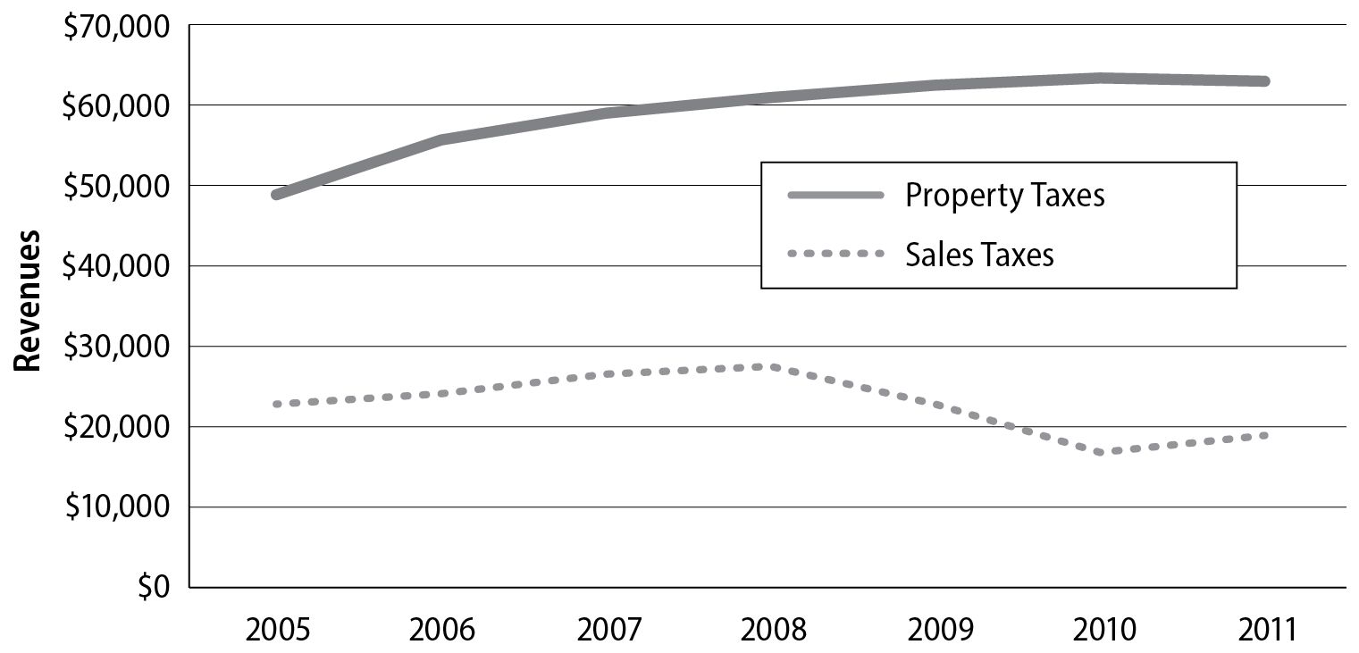
Simply by looking at the revenues generated by these two tax instruments (Figure 6.1), and without applying a formal quantitative methodology, it becomes clear that property tax revenue is more stable³¹ and predictable than sales tax revenue. This reinforces the earlier discussion of needing to forecast revenue sources separately.

Figure 6.1 Alamance County Revenue Collections, by Year

Formula-Based Projections

Formula-based projections, sometimes referred to as deterministic models, are simply mathematical formulas established for estimating future revenues. Once the formulas are created, the forecaster simply needs to plug in the various values required. If a formula-based projection is used, it and any additional information about its accuracy, assumptions, and reliability should be included in a local government’s revenue manual.

The most common formula-based projections made by local governments are property tax forecasts. They often are forecasted according to the following formula:

It would be easy for local governments to forecast their property taxes using the above formula. In fact, it would most likely achieve relatively accurate results. However, it is important to be mindful of collection rates, and in North Carolina the previous year’s collection rate is used in the calculation of property tax forecasts.³² Furthermore, it is important also to incorporate any changes in assessed values into the assessed values used in the calculation of property tax forecasts. This is an excellent example of why the budget director will be updating these projections during this process. New information about collections and property assessments may make the formula look more like the following:

For a local government considering changing its property tax rate, it is fairly apparent how changing the rate would change the amount of revenue collected.

So, for example, had Alamance County officials, in forecasting for FY 2012, used formula-­based projections, they would have forecast exactly what was collected in 2011.³³ This is because they did not change their rate ($0.52 per $100), the last assessment was in 2009, and they are required to use the same collection rate as in the previous year (i.e., FY 2011). So, using formula-­based projections, property tax revenues for Alamance County in FY 2012 would be forecasted at approximately $62,654.

Since all of this information is available to the forecaster for property taxes, this is the most common way to forecast property taxes. Furthermore, it is also highly accurate. For a medium-term forecast, there is no reason to use alternate forecasting methods. However, a local government has the right to choose other forecasting methods. Within this section, alternate forecasting techniques are discussed, property taxes will be used again as an illustrative sample, and the outcomes will be compared to the formula-based projection calculated here. Then they will be compared to actual collections from FY 2012.

Strengths and Weaknesses of Formula-Based Projections

Formula-based projections work best when jurisdictions have a great deal of control over revenue sources³⁴ and those sources are stable, like the property tax, but they work less well for jurisdictions with revenue sources that fluctuate more with the economy, like sales taxes. Formula-based projections are very transparent, with their assumptions clearly laid out, which also makes them easier to understand. However, again using property taxes as an example, the method’s weaknesses include not considering changes in assessments, as when new properties are added or property defaults occur. Fundamentally, formula-based projections are good for property taxes at the local level but not for more-dynamic revenues with harder to characterize (and less stable) tax bases.

Trend Analysis

Trend analysis, also referred to as time-series analysis, captures a great many methods for forecasting. It can include anything from a naive model, where the forecast is simply equal to the previous year’s revenue, to an ARIMA (auto-regressive integrated moving average) model, which is as complicated as it sounds! Within this section, the discussion is limited to two basic trend analysis models: moving averages (three forms are discussed) and univariate regression. Also included is a brief discussion of a cumulative experience curve, which is often used for updating forecasts.

Moving Averages

The moving averages model captures a great many methods for forecasting. One method is simply to project that revenue will increase or decrease by the average amount it has changed over the past five years, thus giving no additional weight to recent years. A forecaster could also forecast the revenue as the average of those years. These decisions often involve assuming that the revenue source is too volatile to reasonably expect a trend to continue upward or downward.

The first form of moving averages, a simple moving average (SMA), is a method wherein the forecaster takes an average of historical data and uses the result as the forecast. In the initial step, the forecaster sets a window for how many years to include in the average (for the purposes of this chapter, a seven-year window is used). After the window is set, the necessary data are collected. (Of course, this is often not the order in practice, as data availability can determine the size of the window.) Once the window is identified and the revenue data are collected, the forecaster takes all of the years of data, sums them, and then divides by the number of years. The reason the result is called a “moving” average is that the next year, the forecaster will drop the most-distant year included and replace it with the current fiscal year’s data. So, it will always be the same number of years, just shifting forward (or moving).

For example, take the property tax revenue from Alamance County and imagine that the forecaster is creating a forecast for FY 2012.³⁵ Using the most-current data (up to and including FY 2011) reported by the North Carolina Department of the State Treasurer (2014), the seven-­year window consists of FY 2005 to FY 2011. A simple moving average forecast for FY 2012 is accomplished by calculating the following:

Imagine changing how large the window is, that is, how many years of historical data are being used. What happens when the window is only six years (so you drop 2005)? Five years? This should illustrate another point: that simple moving averages, like all trend forecasting, are sensitive to the size of the window the forecaster uses. Another weakness is that these moving averages treat the predictive power of previous years the same no matter how recent they are or how far in the past they are.³⁶

The second form of moving averages is arithmetic mean return (AMR). The forecaster using AMR is most interested in calculating the growth rate, which, as defined here, is the percentage increase (or decrease) in collected revenue from the previous year.³⁷ Under this definition, the growth rate for FY 2006³⁸ is calculated as

This means that in FY 2006, Alamance County collected 115 percent of the revenue that was collected in FY 2005.³⁹ The growth rate is calculated as follows:

This is done each year within the specified window. Results are reported below. Then, just like above, the growth rates are averaged.

Thus, the average growth in revenue from FY 2006 to 2011 is 4.5 percent (see Table 6.3).

Once again, the forecaster could simply use the average revenue collected, $58,761, as the forecast for next year. However, what is more likely to be accurate is to take FY 2011 property tax collections ($62,654) and apply the average growth rate of 4.5 percent, which would result in an estimate of $65,473.43 for FY 2012. Some questions to consider are the following: Do any of the numbers stand out? Looking at the data and not just the calculations, does it seem reasonable to expect a 4.5 percent growth rate? Not really. The growth rate for property taxes decreased dramatically in 2007 and has continued to slow. In fact, by removing the change between FY 2005 and 2006, the average growth rate drops from 4.5 percent to 2.5 percent, which, in light of the trend, seems more likely. A forecaster for Alamance County might have been even more cautious and noted that property taxes experienced negative growth in the most recent year.

Third, a forecaster can create moving means that, once calculated, can be used with either simple moving averages or the AMR technique. Using the moving means method, the forecaster calculates an average for each year by, for example, taking the average of the year in question, the year before it, and the year after it. Then, using the three-year average as the value for that year, the forecaster conducts the same trend analysis as above. This method helps smooth bumps and “noise” from the estimates. So, if one year the revenue was particularly high or low, the influence of that data point can be minimized without it actually being removed from the analysis.

Again plugging in the property tax revenue data from Alamance County, the data point to be used for FY 2006 using a three-year window is calculated by taking the average for fiscal years 2005, 2006, and 2007.

A forecaster who wanted to use moving means with a simple moving average could replace the actual revenue collections with these smoothed estimates. The calculation would include estimates for FY 2006 through 2010. Another option, which adds a slight weight to recent data, is to use the FY 2011 data but, because the forecast is for FY 2012, use the average of 2010 and 2011. This weights the two most-recent years more heavily than the previous years, which are averages of three years. That is accomplished as follows.

In contrast to using just the simple moving average, the above formula results in a higher revenue forecast: $60,114.58 versus $58,761. Of course, the goal is not to forecast the most revenue but, rather, the most accurate. When looking at the trend in recent years, this still appears to be a conservative estimate.

Similarly, a forecaster can take the transformation moving averages using the moving means. That calculation would look like

So, the expected growth using transformation moving averages in conjunction with moving means produces an expected property revenue for FY 2012 of $62,654 × 1.03 = $64,533.62. This is less than the estimate created by the transformation moving averages above, $66,181.49. This is because the $65,473.43 estimate smoothed some of the more-dramatic changes.⁴⁰

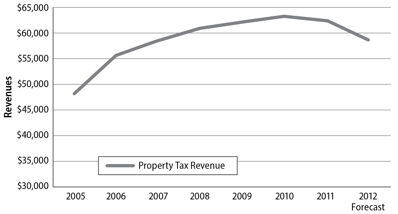
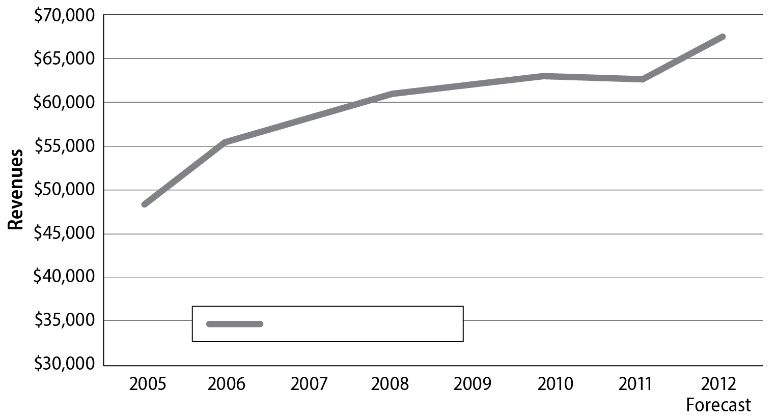
Once again it is helpful to look at these forecasts visually (where expert judgment is useful). Using the simple moving averages method (Figure 6.2), it is apparent that there is expected to be a relatively sharp decline in property tax revenue in FY 2012. This is unlikely and would often be considered too conservative.

Figure 6.2 Simple Moving Averages: Property Tax Revenue

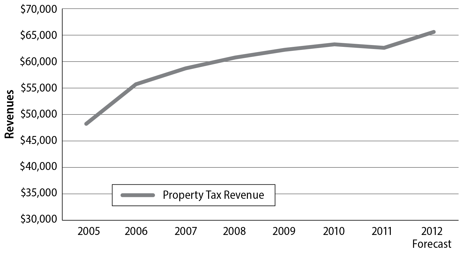
In contrast, when looking at the revenue forecast created by the estimate of 4.5 percent growth (Figure 6.3), it is clear that it has forecasted a relatively sharp increase in property tax revenue for FY 2012. This is likely going to be considered by a finance or budget officer as too ambitious of an estimate. That is, unless the finance/budget officer applies their expert judgment and considers that growth has been slowed by the recession and that their county is expecting to start a nice rate of recovery.

Figure 6.3 Arithmetic Mean Return: Property Tax Revenue

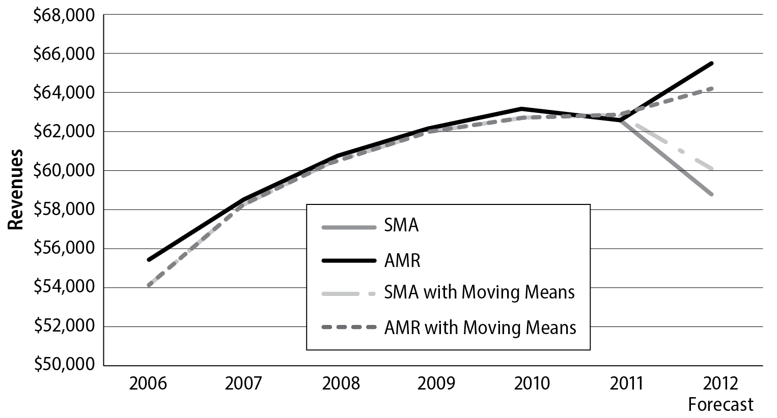
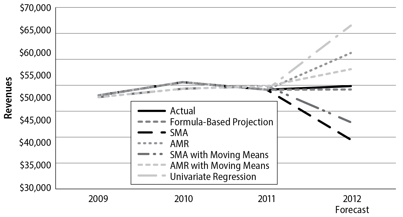
Below are the forecasts for the simply moving averages (SMA) and for arithmetic mean return (AMR) using the moving means (Figure 6.4). As is apparent under both approaches, moving means do, in fact, smooth the estimates and present what is most likely a more-­accurate forecast of revenue. It still seems likely, though, that one is too conservative and the other too optimistic.

Figure 6.4 Forecasted Revenues Using Moving Means

Univariate Regression

A simple way to forecast revenues using a statistical model is through univariate regression. Univariate simply means that only one independent (or control) variable is being used to predict the dependent variable. So, in the example we’ve been using, the independent variable is years and the dependent variable is revenue collections. The software captures the relationship between time progressing and revenue collections.

This model can be presented as y = ∝ (x) + β, where y is the dependent variable, x is the independent variable, ∝ is the slope of the line when graphing it, and β is a constant term (or the point where the slope of the line intercepts with the y-axis on a graph). ∝ is how much revenue is forecasted to increase (or decrease) from the previous year based on earlier trends. Once again, some level of expert judgment is needed to confirm that there are no meaningful changes on the horizon that would affect future collections.

In this context the model can also be written as

Univariate regression can be performed in many statistical packages, including Microsoft Excel. Here is a tip for forecasting revenue this way: look for a high R, or the correlation coefficient. R, which will be reported with the results, is measured on a scale from 0 to 1, where an R of 0 suggests no correlation and predictive ability and an R of 1 suggests perfect predictive ability. Neither situation is likely.

Reported here are estimates that are generated by performing univariate regression in Excel. The Excel regression estimates the constant⁴¹ to be $49,898.14 and the ∝ to be $2,215.71.⁴² In order to forecast for FY 2012, the forecaster would use these estimates in the above equation:

Eight is used as the variable for the year because it is the eighth year of data in the window. This is only the case because the years for the regression were changed from 2005 through 2011 to 1 through 7. If left as is, the ∝ would have been much lower and 2012 would have been the appropriate multiplier.

In addition, the output produces an R of 0.90, so there is a great deal of predictive ability based on the time trend alone.

Once again, the forecast methodology has predicted a relatively sharp increase, in fact the largest so far (Figure 6.5). This is due to the trend of the data. The recession slowed what had been steady growth, so the forecasting methods are picking up on the earlier trend and dampening it by the slowed (and, in FY 2011, negative) growth. This clearly demonstrates, once again, the importance of always integrating some level of expert judgment into all methods.

Figure 6.5 Univariate Regression: Property Tax Revenue

Which method is most accurate for forecasting property taxes? According to the Alamance County budget for FY 2014, property tax revenue was $62,961 in FY 2012.⁴³ It is clear that for a one-year property tax forecast, formula-based projection is the most accurate method. (See Figure 6.6 for a visual representation of all of the methods, including the actual revenue collected in FY 2012 for property taxes.) Now try replicating these methods for sales taxes. What stands out? Does either type of moving averages seem more reasonable for sales taxes than for property taxes? Moving means? Compare the sales tax forecasts with the actual FY 2012 revenue, which is: $17,328.

Figure 6.6 Forecasted Property Tax Revenue

Cumulative Experience Curve

A third method of trend analysis is the cumulative experience curve. It is used most frequently to modify projections as revenue comes in during the fiscal year. Using a cumulative experience curve the forecaster examines monthly totals of revenue collected over a five-year period.⁴⁴ The forecaster takes the average amount collected per month and converts it into a percentage of the total amount of revenue collected. Then, once actual collections for the month in the current fiscal year are known, the forecaster can modify projections for the rest of the year. Of course, this is true only if the forecaster is willing to assume that the percentage of the total will be approximately the same. Ideally, this would be done by a local government throughout the year with the time frame and expectations clearly laid out in the unit’s revenue manual.

Strengths and Weaknesses of Trend Analysis

As has been noted, a forecaster should always incorporate a level of expert judgment into creating forecasts. One reason for this is that trend analysis is fundamentally based on the idea that the past can be used as a good predictor of the future. However, if a community has experienced large economic shocks or changes this will not hold true. While these trend analyses can be valuable, research suggests that this method is most effective when used in combination with expert judgment.⁴⁵ The greatest weakness of trend analysis is not being able to anticipate coming changes or incorporate known changes into the model. This results in forecasts lagging behind changes to the economy.

Nonetheless, trend analysis is largely accurate for more-stable revenue sources. It also requires modest data and is relatively straightforward to implement. This is one reason why it is used heavily by smaller local governments.⁴⁶

Causal Modeling

Causal modeling, also referred to as econometric modeling or multiple (multivariate) regression, models the “relationship between the revenue source and the economic variables that drive the tax base; in other words, this approach looks for what causes the collections to be what they are and creates a model of the relationship.”⁴⁷ Causal modeling recognizes that demographic and economic changes to a community affect its revenues. These could include such factors as population, median income, inflation, and industry. It allows a forecaster to take data on an individual local government and determine how tax revenue is expected to change when a component of the model changes, for example, when unemployment increases, and how it is expected to affect a revenue source. Causal modeling becomes more valuable as the size and/or complications of the government, its respective economy, and its revenue portfolio grow.⁴⁸

The section above on univariate regression uses a simple regression equation. To help explain causal modeling, that equation is going to be expanded. The dependent variable, y, continues to be actual revenues over multiple years; however, additional x’s, or independent variables, have been added. The forecaster is going to be predicting revenue based not just on the passage of time, but on its relationship with other variables. In this multivariate model revenues are dependent on these other independent variables, such as unemployment, median income, year, among others (represented by the x’s below). The model can be represented by the following:

Once the model is carefully constructed and the data are input, the forecaster can generate the estimated effect of the independent variables on revenue and make assumptions (possibly from trend analysis or from expert judgment) about those independent variables, use the slopes or the coefficients (like ∝), multiply the projected values for those independent variables, and add the constant term (β) to get their projected revenue.

Below is a description of an academic exercise in forecasting and how the scholar chose to test forecasting methods.

1. The model employed in this article identifies explanatory variables in four areas: personal income, employment, population, and inflation. From each of these four areas, multiple explanatory variables are identified. The personal income area considers county personal income, state personal income, county personal income growth rate, and county per capita personal income as candidates for explanatory variables; the employment area considers county total employment, county total unemployment, county total labor force, county unemployment rate, and state unemployment rate; the population area considers county total population and county population growth rate; and the inflation area considers the national prime interest rate, the national mortgage interest rate, the California consumer price index (CPI) for all urban customers, and the California CPI growth rate. . . . County explanatory variables are forecasted in the simplest way, mainly because including more elaborate forecasting equations for these variables would easily double the size of this model without significantly increasing the overall forecasting accuracy.⁴⁹

This passage should clarify two aspects of causal modeling. First, that it requires a great deal of annual (if not quarterly or monthly) data. This level and quality of data are often difficult to come by, if not impossible. Using data from the last U.S. Census is simply inadequate. Second, in an applied analysis, while Dongsung Kong finds that causal modeling is effective and accurate, he also finds that sparser specifications are accurate. So, it may not be necessary to have all of these variables.

Causal models are used less frequently at the local level and can be very complex and challenging to implement. They are also very sensitive to specification and assumptions about the economy, so the forecaster must take particular care in identifying the independent variables to be included. In addition, as with univariate regression, the forecaster wants to generate a high (close to 1) R-squared. The lower the estimated R-squared, the less predictive power the model has and the less accurate it should be expected to be. An R-squared of one means that all variation between the values of the dependent variable is captured or explained by the covariates in the model, whereas a 0 would mean that none of the variation in the dependent variable is explained by the model.

Strengths and Weaknesses of Causal Models

The primary reason forecasters undertake causal modeling is that it allows for taxes, which are more sensitive to the changing economic environment, to be forecasted based on those changes. This means that causal modeling is more likely to capture shocks and trends. With causal modeling it is not necessarily the case that revenue forecasts will lag behind changes to the tax base in the way they do with trend analysis.

The reason not every local government forecasts using causal modeling is that it is very difficult to do. Most local governments that use this methodology do not do it themselves. They hire economists from either a local university or a consulting firm. In addition, there is often very incomplete data, and “the absence of data on economic and structural variables at the city level” is very restricting.⁵⁰ Many of the key variables that are needed, such as personal income and population, are not available annually and potentially are not even collected for a unit of government (some data are collected just for counties; other data, just for large municipalities or even metropolitan statistical areas). Furthermore, causal models require the forecaster to also estimate the values for the independent variables in the next fiscal year. This introduces the possibility for even more error in the model. These factors make causal modeling difficult if not impossible for many local governments to use.

Overall Assessment of Quantitative Methods

In closing, quantitative forecasting methods may more accurately model future revenues than qualitative methods. When using data, it is always important to remember: garbage in, garbage out. Reliable data is critical. In addition, evidence suggests that the simple, straightforward models perform as well as the complicated models. In both the short and medium term, trend analysis models perform better than causal models. So, it should not be considered necessary for local governments to embark on heroic efforts to perform sophisticated causal models if it is not within their means and the trend analyses have been reliable for them.

Considerations on Choosing the Right Method

There are many factors to consider in determining what method of forecasting is best. In this section some of the more universal factors are discussed, recognizing, however, that a local government can modify these perspectives in light of its own needs, for example, in terms of local capacity and what is realistic. What the forecasting staff (or the lack thereof) are capable of doing, especially with regard to the use of quantitative methods, is a crucial consideration. There is always the question of the budget and if a local government can afford to hire experts to aid in or perform qualitative or quantitative forecasting or if that money could be better used elsewhere. In general, local governments rely heavily on expert judgment (internal and external). More than half of all counties in California, according to one study, use expert judgment as their primary method of forecasting revenues. This is especially true for small jurisdictions, where the number is closer to two-thirds.⁵¹

A forecaster should also carefully consider individual revenue instruments, that is, specific taxes, fees, and the like. Typically, a revenue forecast is created for every major revenue source (so possibly property taxes, sales taxes, and utilities). For the smaller revenue sources a local government may just look at historical numbers and establish an estimated total for each source. Even within that context, however, the same forecast method is most likely not the best choice for all of the revenues to be forecasted.

Therefore, it becomes important to ask how a forecaster decides to choose between the available methods. First, the data are examined for trends, patterns, and rates of changes. An important component of this process is considering how stable the revenue source is, not just the “trend” but how closely it follows that trend.⁵² Sales taxes are more unstable than property taxes, and this makes trend analysis more problematic in light of the cyclical nature of the economy. For example, “property taxes for most local governments are levied on an assessed value base that, because of assessment lags, is known at the time that budgets are adopted and property tax rates are set, [but] there [are] no such lags for sales and income taxes; their bases are emerging as the budget is being executed.”⁵³ Therefore, a formula-based forecast or a trend analysis may be best suited for property taxes, and a causal model may best capture sales tax revenue forecasts.

Examining the economic, political, and social influences on a particular revenue source can also be useful. Look beyond the data. Is the revenue instrument, or more accurately its base, likely to be affected by a recession? Is citizen demand for this service growing? Some of these relationships and assumptions will help guide you to the appropriate forecasting method.⁵⁴

A third way of approaching the potentially difficult decision of selecting the proper forecasting method is simply to forecast the most recent complete year of revenue using the competing methods and see which ones work best for which instruments, as has been done here. There is an online resource included with this chapter. It presents an Excel spreadsheet and step-by-step directions for recreating the different forecasting methods highlighted in this chapter. This resource is a good initial step for a new forecaster or for someone who is reconsidering which forecasting method might work best for the revenue instrument they are responsible for forecasting. It is advisable to begin with the revenues presented here to ensure that the forecasted amounts are equivalent and that the methods are clear. A forecaster could then insert their own revenue values to begin the analysis for themselves.⁵⁵

Finally, a forecaster may also want to know what forecasting method has been found to be the most accurate by academic researchers. Unfortunately, such studies do not provide a consensus view. Some studies have found that simple time-series models, particularly the moving average, produce the most reliable results.⁵⁶ Another study, however, found that judgmental methods perform better than time-series or causal models.⁵⁷ A more-recent study found that, when looking at sales taxes, causal models perform best and trend analysis does poorly even though it is the most common of those being tested.⁵⁸ In addition, that study found that “simpler, more readily communicated models generally perform at least as well as more complex methods.”⁵⁹

Best Practices in Forecasting Revenues

There are many best practices when it comes to forecasting, many of which have been mentioned in this chapter. This section focuses on many of the more-successful practices. By no means is this an exhaustive list, however, and not every method is necessarily best for every local government.

The first best practice is to create a revenue manual (described as step 1 in the section above titled “Potential Administrative Process for Revenue Forecasting”). This is an action that all local governments should be able to take and that should be of universal benefit. If a local government does not already have a revenue manual in place, the process of creating one may be a multi-year undertaking. The place to start is at the top, with major revenue sources.

Second, forecasters should consider creating hybrid or conditional models that can be adjusted in line with other scenarios, such as changes in tax rates or the tax base.⁶⁰ For example, adjusting the tax rate is a straightforward process in a formula-based allocation.⁶¹ In fact, one of the common uses of forecasting beyond creating one-year revenue projections for a local government’s budget is guiding tax-rate adjustments. This is helpful in trying to establish consistent tax policies so that tax rates do not have to be adjusted every year.⁶² This is best when the process is transparent and the assumptions are clearly laid out. Hybrid models present alternative forecasts of possible revenues, act as a sensitivity test to assumptions in the model, and provide elected officials with options if they are considering changing elements of their policy.

It is important to remember that forecasts are projections, not predictions. While a hybrid model may be useful in testing assumptions and providing options and, in some cases, for assisting in long-term planning, it is not appropriate or acceptable for annual budget forecasts. Revenue numbers must be decided upon and used to balance the budget.

Third, be careful when managing the data. Below are three tips for dealing with the data used to make forecasts.⁶³

1. Always graph data. This allows for a deeper understanding of what the data are saying and ensures that the data make sense in the context of institutional knowledge.

2. Adjust away outliers. Some data points will not be representative. A graph helps identify such cases so that they can be removed or handled differently, for example, by using moving means.

3. Keep records of original, unadjusted data. It is a best practice to always keep a file with the original data before it has been modified, adjusted, or manipulated. This allows one to go back and see what the data said before adjustments were made, to look for patterns that might have been missed or that are new, for example, that an outlier was not an outlier but actually the start of a new event or period.

Fourth, consider other factors beyond the revenue forecasts that may be affected by their accuracy, for example, a local government’s fund balance. It is clear that revenue projections or forecasts are not going to be completely accurate, and while it is considered best to err slightly on the conservative side of forecasting, it should nonetheless be apparent that this is one of the many reasons that maintaining a fund balance is encouraged—not just for downturns, but also for years when estimates are on the high end of the spectrum. This is especially important when there is less confidence in the forecasts. For example, if a forecast relies heavily on sales taxes, and they are volatile historically, a local government may choose to maintain larger fund-balance reserves.⁶⁴

Fifth, create within-year monthly or quarterly targets for periodic revenues, such as sales taxes. These should be based on historical data, typically a three-year average monthly (or quarterly) collection number that reflects the expected trend for that year. So, if one-eighth of all local sales tax revenue is collected in November, on average, the target for November should be approximately one-eighth of what has been forecasted for the year.

Sixth, consider creating a long-term financial plan. The National Advisory Council on State and Local Budgeting (NACSLB) encourages local governments to develop such a plan by using a strategic process that allows for greater insights and the information necessary to establish policies surrounding both expenditures and revenues that will lead to long-term fiscal health.⁶⁵

Finally, as noted in the section on choosing the right forecasting method, one should consider how a given revenue source is likely to be impacted by changes in the broader economy, such as a recession. The twenty-first century has demonstrated that taking stock of the cause of a recession and its anticipated impact on the economy more broadly must also be integrated into the forecasting process. In the past, it was reasonable for a forecaster operating in the midst of a recession or out of concern that one may be on the horizon to turn to previous economic downturns to inform revenue projections. As evidenced by the tremendous diversity in the three recessions of this century (the dot-com recession of the early 2000s, the Great Recession, and the recession brought on by the pandemic), it is clear that the underlying cause of a recession is critical to understanding how it impacts revenues.⁶⁶ The dot-com recession behaved similarly to past recessions, as did the Great Recession in many respects, but the severity, length, and impact of these two events on property taxes were largely unprecedented. The pandemic-­induced recession behaved very differently from the other two twenty-first century recessions and had forecasters during this time used numbers and trends from the Great Recession, it would not have led to accurate forecasting.⁶⁷ Trend analysis would not be able to factor in these differences or the concern of a looming economic downturn. Once again, this is where expert judgement is critical to forecasting.

Forecasting Is Not Perfect

It is important to remember that no forecast is ever completely accurate; the numbers will inevitably be wrong. The goal is to minimize how wrong they are! With that in mind, there are four additional points to be made about errors in forecasting.⁶⁸ First, the forecaster should strive to include predicted errors with the estimates. It should be clear how confident the forecaster is that these forecasts are reliable. Second, the farther out the forecast, the larger the errors are likely to be. Third, forecasts are built upon the past. This has two important implications: (1) if the future deviates from the past in a meaningful way the forecasts will not be accurate and (2) if key data or trends from the past are ignored, more errors will be introduced into the estimates. Fourth, forecasting for a period greater than three years will be more reliable if the revenues are more aggregated. So, while it is useful to forecast individual revenue streams for the short and medium term, this is less valuable for long-term forecasting.

Because errors do inevitably occur, it is advisable to forecast on the conservative side, but just slightly so. It is not prudent to dramatically underestimate revenues because budgets do have to be balanced, which could cause budget makers to make unnecessary cuts to services or to increase taxes. “Estimates that are too high can create major crises during the execution phase, at which time expenditures must be cut so as not to exceed revenues. Low estimates also cause problems, in that programs may be needlessly reduced at the beginning of the fiscal year.”⁶⁹

Forecasting: Cautions

Beyond just the reliability of the results produced by a methodology, time frame, and data, other concerns may corrupt a forecaster’s estimates, for example, when politics enters the process. Unfortunately, forecasting can quickly become political. This is why, in general, it is often considered a best practice to be slightly conservative and to estimate revenues just below where the forecaster thinks they will be.⁷⁰ However, this practice makes it harder to balance the budget and may require service cuts or increased taxes, so it is also possible that forecasters will face pressure to be more optimistic. It is important to stand your ground though, because “in revenue forecasting, your sins find you out, and they do have a cost.”⁷¹

Another persistent problem in generating reliable forecasts is the cyclical nature of the economy. Taken back far enough, historical data reveals periodic dips in growth. Revenues, some more than others, are cyclical and influenced by business cycles, which can be understood as natural expansions and recessions (shrinking) of the economy.⁷² As local governments reduce their reliance on property taxes and increase their use of user fees and sales taxes, awareness of this will become even more critical. Keep this in mind as forecasts are prepared, especially for long-term forecasts.

Conclusion

Revenue forecasting is an exercise that every local government performs. Despite that universality, there is a great deal of diversity in the methodology of those forecasts—some local governments may choose to simply forecast next year’s revenue to equal the previous year’s revenue, whereas others may create sophisticated causal models that attempt to capture the changing nature of the underlying tax base. These potential extremes highlight the need for transparency both internally and externally. Revenue forecasts should not just provide a number; they should also (especially if quantitative) provide the methodology and assumptions on which forecasts are based. One place for a local government to record this information is in a revenue manual.

In addition, local governments need to be thoughtful when choosing which forecasting methods are best for them and when they should employ different methods for different revenue instruments. Unfortunately, there is no one right answer. The benefit of having a more-advanced forecasting method with slightly more-accurate forecasts may not outweigh the additional costs of performing it.⁷³ These costs may be direct, such as paying outside consultants, or indirect, such as staff time and additional training. In light of the information presented in this chapter, it should not be surprising that expert and trend analyses are the most-common methods for forecasting revenues and expenditures in North Carolina and that there is no standard model or methodology because each local government develops its own catered to its particular needs.⁷⁴

Although revenue forecasting may seem like, and often is, a challenging undertaking, there are many excellent resources available to local governments in North Carolina.⁷⁵ Below are resources to enable budget and finance officers to reach out and connect with peers and experts.

• North Carolina League of Municipalities (NCLM): www.nclm.org;

• North Carolina Association of County Commissioners (NCACC): www.ncacc.org;

• North Carolina Government Finance Officers Association (NCGFOA): www.ncgfoa.org;

• North Carolina Local Government Budget Association (NCLBA): www.nclgba.org;

• School of Government (SOG): www.sog.unc.edu.


• Excel spreadsheet on revenue forecasting (prepared by the author) and directions for using the spreadsheet: https://www.sog.unc.edu/pubs/978642380798.

For more on additional forecasting methods and a more in-depth discussion of the math behind revenue forecasting, the following resources may be helpful.⁷⁶

• Thomas A. Garrett and John Leatherman, An Introduction to State and Local Public Finance (Morganton, WV: Regional Research Institute, West Virginia University, 2000), www.rri.wvu.edu/WebBook/Garrett/contents.htm.

• Dongsung Kong, “Local Government Revenue Forecasting: The California County Experience,” Journal of Public Budgeting, Accounting & Financial Management 19, no. 2 (2007): 178–99.

• Gloria A. Grizzle and William Earle Klay, “Forecasting State Sales Tax Revenues: Comparing the Accuracy of Different Methods,” State and Local Government Review 26, no. 3 (1994): 142–52.

• Shayne C. Kavanagh and Charles Iglehart, “Structuring the Revenue Forecasting Process,” Government Finance Review (Oct. 2012), www.gfoa.org/structuring-revenue-forecasting-process.